midasINLA provides tools for fitting mixed-data sampling (MIDAS) regression models using Integrated Nested Laplace Approximation (INLA). The package is designed for settings where the response is observed at a lower frequency than one or more explanatory variables, and supports both constant and spatially varying regression coefficients.
Overview
MIDAS models allow high-frequency covariates to be incorporated into models for lower-frequency responses through weighted distributed lags. midasINLA combines this framework with INLA, allowing MIDAS regression models to be fitted efficiently within a latent Gaussian modelling framework.
The conceptual framework for spatial distributed-lag MIDAS modelling is illustrated in the figure below. High-frequency covariates are linked to lower-frequency responses through weighted distributed lags, with MIDAS coefficients potentially varying across spatial locations.
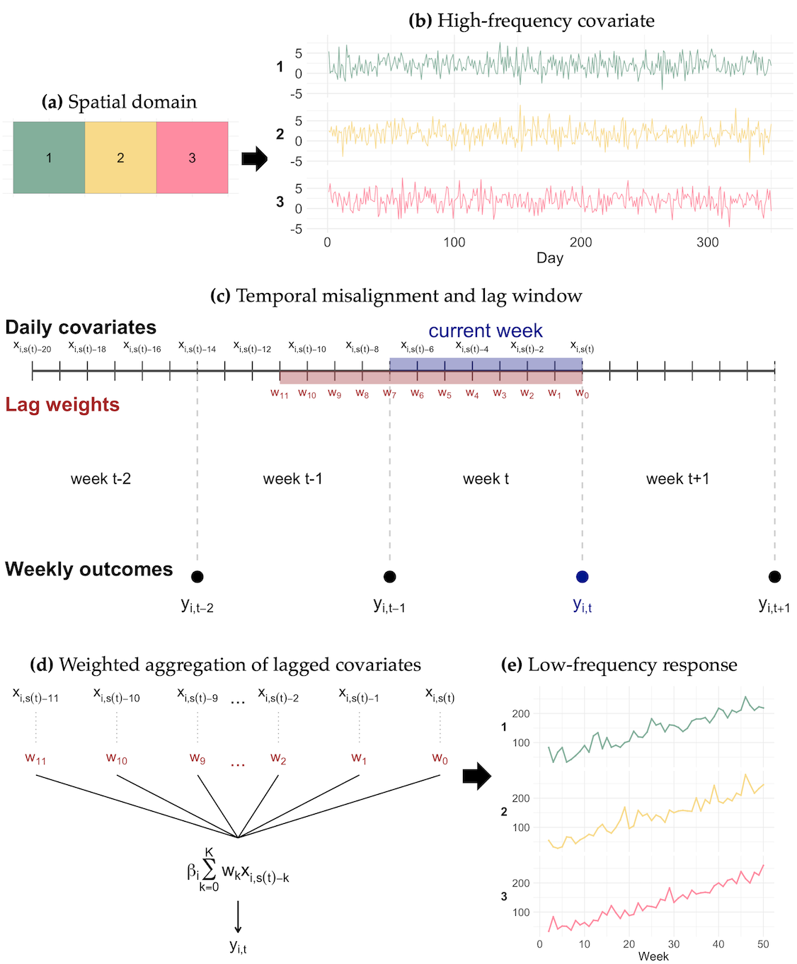
Figure 1. Schematic representation of the spatial mixed-frequency setting and the MIDAS aggregation mechanism. (a) Spatial domain with three areal units. (b) Daily high-frequency covariate processes for each unit. (c) Temporal misalignment between daily covariates and weekly outcomes, with the highlighted lag window corresponding to the covariates used to predict the current weekly response. (d) MIDAS-based weighted aggregation of lagged daily covariates into a low-frequency predictor. (e) Weekly low-frequency response process for each spatial unit.
Installation
The latest released version of midasINLA can be installed from CRAN:
install.packages("midasINLA")The development version can be installed from GitHub using remotes:
if (!requireNamespace("remotes", quietly = TRUE)) {
  install.packages("remotes")
}

remotes::install_github("stephen-villejo/midasINLA")
Getting started
The package includes a spatial Poisson dataset illustrating the main modelling workflow. A typical analysis involves preparing high-frequency covariates, fitting a spatial MIDAS model, and obtaining posterior summaries.
library(midasINLA)
library(INLA)

data("data_spatialpoisson_example")

# Read the spatial adjacency graph
g <- INLA::inla.read.graph(
  filename = system.file("map.adj", package = "midasINLA")
)

# Prepare the first high-frequency covariate
Midas_x1 <- prepare_Minla_spatial(
  x = data_spatialpoisson_example$data_x1$x1,
  loc_x = data_spatialpoisson_example$data_x1$loc,
  constraint = "hyperbolic",
  K = 0:29,
  m = 30,
  svc = TRUE,
  svc_prior = "icar",
  g = g
)

# Prepare the second high-frequency covariate
Midas_x2 <- prepare_Minla_spatial(
  x = data_spatialpoisson_example$data_x2$x2,
  loc_x = data_spatialpoisson_example$data_x2$loc,
  constraint = "gaussian",
  K = 0:45,
  m = 30,
  svc = FALSE
)

# Fit the model
fit_res <- fit_Minla_spatial(
  formula = y ~ 1,
  hf_input = list(Midas_x1, Midas_x2),
  data = response_data,
  loc_var = "loc",
  time_var = "Time",
  family = "poisson",
  inla_options = list(
    verbose = FALSE,
    num.threads = 1,
    control.predictor = list(
      compute = TRUE,
      link = 1
    )
  )
)
Documentation
For a complete walkthrough, including posterior MIDAS coefficients, lag weights, and predictions, see the package vignette:
vignette("midasINLA", package = "midasINLA")Individual functions can also be explored using R’s help system: ?prepare_Minla_spatial ?fit_Minla_spatial ?compute_beta_spatial ?compute_weights ?predict_midas
Applications
midasINLA was developed to facilitate Bayesian modelling of relationships between variables observed at different temporal resolutions, with particular emphasis on applications involving spatial data.
The package is particularly useful in environmental epidemiology, climate–health modelling, and other settings where high-frequency exposures need to be linked to lower-frequency outcomes.